
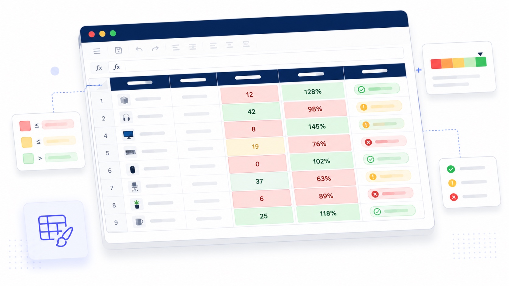
In the cell types article we put interactive controls inside cells. This time we let the grid style itself: stock below a threshold turns red, sales over target turn green, cancelled orders flag automatically — and every one of those colors updates the instant a value changes. No restyling loop, no re-render plumbing. You declare the rules once.
What is conditional formatting?
Conditional formatting applies styles to cells based on their values. You define rules — “if stock < 20, paint it red” — and the grid re-evaluates them on every edit. It’s the difference between a static report and a dashboard that reacts.
ReoGrid Web supports three rule types, the same three Excel users already know:
| Type | Decides by | Example |
|---|---|---|
cellIs | Comparing the value against fixed thresholds | Highlight stock < 20 |
expression | Evaluating a formula per cell | Highlight where =E2>D2 (sales beat target) |
containsText | Matching a substring in the text | Color-code "Cancelled" rows |
Conditional formatting is a Pro feature (pricing). The code below assumes
@reogrid/pro.
The simplest rule
Attach a rule to a range with addConditionalFormat. Arguments are an Excel-style A1 range and a rule object:
import { createReogrid } from '@reogrid/pro';

const { worksheet } = createReogrid('#grid');
worksheet.setGridSize(100, 8);  // the default sheet is 40 rows

// Paint scores of 90 and up green
worksheet.range('C2:C100').addConditionalFormat({
  type: 'cellIs',
  operator: 'greaterThanOrEqual',
  value1: 90,
  style: { backgroundColor: '#bbf7d0', color: '#14532d', bold: true },
});
A sheet starts at 40 rows, and a range that reaches past the last row is dropped without a warning — formats, styles, conditional formats and validation rules all fall silently on the floor. Call
setGridSize()(or size the sheet from your data) before addressing something likeB2:B100.
That’s the whole pattern. Everything else is choosing the rule type and stacking rules.
Worked example: a live inventory dashboard
Let’s build a product table that tells you at a glance what needs attention — low stock in red, healthy stock in green, sales that beat (or missed) target, and status-colored order states. This is the complete code.
import { createReogrid } from '@reogrid/pro';

const { worksheet: ws } = createReogrid('#grid');

ws.suspendRender(); // batch the initial build

// ── Columns ──
[140, 110, 80, 80, 80, 100, 100].forEach((w, i) => { ws.column(i).width = w; });

// ── Data ──
const HEADERS = ['Product', 'Category', 'Stock', 'Target', 'Sales', 'Revenue', 'Status'];
const ROWS = [
  ['Wireless Mouse',      'Electronics', 150, 200, 210, 6300,  'Delivered'],
  ['USB-C Hub',           'Electronics',  25, 180, 165, 8250,  'Delivered'],
  ['Standing Desk',       'Furniture',    45, 100,  82, 24600, 'Pending'],
  ['Ergonomic Chair',     'Furniture',     8,  60,  45, 13500, 'Pending'],
  ['Mechanical Keyboard', 'Electronics', 200, 300, 320, 25600, 'Delivered'],
  ['Webcam HD',           'Electronics',  65, 150,  95, 4750,  'Cancelled'],
  ['Laptop Stand',        'Accessories',   5,  90,  70, 2100,  'Pending'],
  ['Noise-Cancel Buds',   'Electronics',  15, 250, 180, 14400, 'Pending'],
];

// Header row
HEADERS.forEach((h, c) => {
  ws.cell(0, c).setValue(h).setStyle({
    bold: true, backgroundColor: '#1e3a5f', color: '#e2e8f0', textAlign: 'center',
  });
});
ws.row(0).height = 30;

// Data rows (numbers right-aligned)
ROWS.forEach((row, r) => {
  row.forEach((val, c) => {
    ws.cell(r + 1, c).setValue(val).setStyle({ textAlign: c >= 2 && c <= 5 ? 'right' : 'left' });
  });
});

const last = ROWS.length + 1; // last 1-based row index

// ── Rule 1: Stock — a traffic light (cellIs + priority + stopIfTrue) ──
ws.range(`C2:C${last}`).addConditionalFormat({
  type: 'cellIs', operator: 'lessThan', value1: 20,
  priority: 1, stopIfTrue: true,
  style: { backgroundColor: '#fecaca', color: '#7f1d1d', bold: true }, // critical
});
ws.range(`C2:C${last}`).addConditionalFormat({
  type: 'cellIs', operator: 'lessThan', value1: 50,
  priority: 2, stopIfTrue: true,
  style: { backgroundColor: '#fef3c7', color: '#92400e' },             // low
});
ws.range(`C2:C${last}`).addConditionalFormat({
  type: 'cellIs', operator: 'greaterThanOrEqual', value1: 150,
  priority: 3,
  style: { backgroundColor: '#bbf7d0', color: '#14532d', bold: true }, // healthy
});

// ── Rule 2: Sales vs Target — formula-based (expression) ──
ws.range(`E2:E${last}`).addConditionalFormat({
  type: 'expression', formula: '=E2>D2',          // beat target
  priority: 1, stopIfTrue: true,
  style: { backgroundColor: '#dcfce7', color: '#166534', bold: true },
});
ws.range(`E2:E${last}`).addConditionalFormat({
  type: 'expression', formula: '=E2<D2*0.7',      // under 70% of target
  priority: 2,
  style: { backgroundColor: '#fee2e2', color: '#991b1b' },
});

// ── Rule 3: Status — text matching (containsText) ──
ws.range(`G2:G${last}`).addConditionalFormat({
  type: 'containsText', operator: 'contains', text: 'Delivered',
  style: { backgroundColor: '#dcfce7', color: '#166534' },
});
ws.range(`G2:G${last}`).addConditionalFormat({
  type: 'containsText', operator: 'contains', text: 'Cancelled',
  style: { backgroundColor: '#fee2e2', color: '#991b1b', bold: true },
});

// ── Rule 4: High revenue — bold blue, no fill ──
ws.range(`F2:F${last}`).addConditionalFormat({
  type: 'cellIs', operator: 'greaterThanOrEqual', value1: 10000,
  style: { bold: true, color: '#1d4ed8' },
});

ws.range(`A1:G${last}`).border({ style: 'solid', color: '#cbd5e1' });

ws.resumeRender();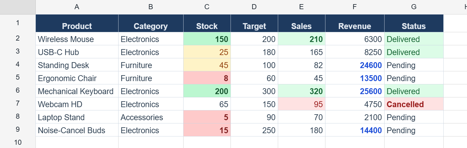
That’s a four-color dashboard from four blocks of declarations. A few things worth calling out.
cellIs — comparing against thresholds
The workhorse. Compare each cell against one or two fixed values:
// One threshold
ws.range('C2:C100').addConditionalFormat({
  type: 'cellIs', operator: 'lessThan', value1: 50,
  style: { backgroundColor: '#fef3c7' },
});

// Two thresholds (a band)
ws.range('C2:C100').addConditionalFormat({
  type: 'cellIs', operator: 'between', value1: 50, value2: 70,
  style: { backgroundColor: '#fef3c7' },
});
The operators map one-to-one to Excel: equal, notEqual, greaterThan, lessThan, greaterThanOrEqual, lessThanOrEqual, between, notBetween. The two-value operators (between / notBetween) read both value1 and value2; the rest use value1 only.
expression — when a comparison isn’t enough
A cellIs rule can only look at the cell it’s coloring. To compare two columns — sales against target — you need a formula. Write it for the first row of the range, and ReoGrid offsets the relative references down each row automatically:
// Color column E green where Sales (E) beats Target (D)
ws.range('E2:E100').addConditionalFormat({
  type: 'expression',
  formula: '=E2>D2',   // evaluated as E3>D3, E4>D4, … down the range
  style: { backgroundColor: '#dcfce7', color: '#166534', bold: true },
});
The leading = is optional — 'E2>D2' works identically. Anything the formula engine can evaluate is fair game, so you can fold in functions: =AND(E2>D2, G2="Delivered").
containsText — color-coding text
For status columns, match a substring. Matching is case-insensitive by default (Excel-compatible):
ws.range('G2:G100').addConditionalFormat({
  type: 'containsText', operator: 'contains', text: 'Cancelled',
  style: { backgroundColor: '#fee2e2', color: '#991b1b', bold: true },
});
Text operators are contains, notContains, beginsWith, endsWith. Pass caseSensitive: true when you need an exact case.
Priority and stopIfTrue — the traffic-light trick
When several rules target the same cell, priority sets the evaluation order (lower number first), and stopIfTrue halts evaluation once a rule matches. Together they give you “first match wins” — exactly what a traffic light needs, so a critically-low value doesn’t also pick up the “merely low” yellow:
// stock < 20 → red, and STOP (don't also apply the yellow rule below)
ws.range('C2:C100').addConditionalFormat({
  type: 'cellIs', operator: 'lessThan', value1: 20,
  priority: 1, stopIfTrue: true,
  style: { backgroundColor: '#fecaca' },
});
// stock < 50 → yellow
ws.range('C2:C100').addConditionalFormat({
  type: 'cellIs', operator: 'lessThan', value1: 50,
  priority: 2, stopIfTrue: true,
  style: { backgroundColor: '#fef3c7' },
});
// stock >= 150 → green
ws.range('C2:C100').addConditionalFormat({
  type: 'cellIs', operator: 'greaterThanOrEqual', value1: 150,
  priority: 3,
  style: { backgroundColor: '#bbf7d0' },
});
Without stopIfTrue, later matching rules stack on top — sometimes what you want (a fill and a bold-blue text rule), sometimes not.
It re-evaluates itself
The payoff: rules are live. Change a cell and the grid re-runs every rule that covers it — by hand, by formula, or programmatically:
ws.cell('C5').value = 12; // drops below 20 → the cell turns red on its ownThis is what makes a ReoGrid sheet a dashboard rather than a snapshot. Wire the values to your data source and the colors follow the numbers with zero extra code. Try it in the conditional formatting demo: edit the Stock and Sales columns, or hit “Randomize,” and watch the whole grid recolor.
Bonus: colored borders
Beyond a style payload, a rule can carry a border payload that paints individual edges — handy for flagging an outlier with a colored rule without disturbing the rest of the cell’s look:
ws.range('B2:B100').addConditionalFormat({
  type: 'cellIs', operator: 'greaterThan', value1: 1000,
  style: {},  // style is required — pass {} for a border-only rule
  border: { right: { style: 'solid', color: '#dc2626', width: 2 } },
});
Omit a side to leave its manual border untouched. style and border combine — both apply when the rule matches.
Managing rules
const id = ws.range('C2:C100').addConditionalFormat({ /* … */ }); // returns an id

ws.removeConditionalFormat(id);            // remove one rule
ws.range('C2:C100').clearConditionalFormats(); // clear a range
ws.clearConditionalFormats();              // clear the whole sheet
ws.getConditionalFormats();                // list: [{ id, range, rule }, …]
Where Lite ends and Pro begins
| Operation | Lite (free) | Pro |
|---|---|---|
| xlsx import, merges, borders, number formats | ✅ | ✅ |
Arithmetic formulas (=D4*1.25) | ✅ | ✅ |
Conditional formatting (addConditionalFormat) | — | ✅ |
Built-in functions (SUM, COUNTIF, …) | — | ✅ |
xlsx export (saveAsXlsx) | — | ✅ |
Displaying, editing, and loading xlsx all work in the free Lite tier. Rule-based styling that re-evaluates itself is where Pro begins.
xlsx round-trip
Rules survive the round trip to Excel. On export they’re written as standard <conditionalFormatting> elements with styles in the <dxfs> table; per-side border payloads round-trip through <dxf><border>. Open the file in Excel and the same rules are right there in Home → Conditional Formatting → Manage Rules — and re-importing brings them back into the grid.
Wrapping up
Conditional formatting turns a table into something that reads itself. Three rule types — cellIs for thresholds, expression for cross-column logic, containsText for status — plus priority / stopIfTrue for traffic lights, and the grid keeps every color in sync as values change.
See it live in the conditional formatting demo, or read the full API in the conditional formatting docs. For drawing interactive UI inside cells instead of styling them, see the cell types article.